3 Sample QC
Compiled: 2025-05-08 Written by Shuting Lu and Daihan Ji
library(SingleCellMQC)
#Load a pre-existing Seurat object or process raw data using SingleCellMQC.
pbmc <- readRDS("/data/pbmc.rds")
The main tasks of sample-level QC include:
- Sample quality assessment- Detecting technical artifacts that may caused by library construction, insufficient sequencing depth, amplification biases, and contaminations;
- Outlier sample detection- Identifying outlier samples with low cell counts, poor RNA quality, or unexpected cell type compositions, et.al;
- Sample identity verification- Recognizing incorrect sample labeling that might be caused by errors in sample handling.
Calculating sample metrics before QC
SingleCellMQC simplifies the process of calculating multi-omics metrics for sample quality control, enabling researchers to efficiently assess data quality before proceeding with downstream analysis. It offers a comprehensive suite of QC metrics designed to evaluate single-cell data quality at the sample level, covering diverse modalities such as RNA sequencing, surface protein profiling (ADT), and TCR/BCR sequencing.
3.1 Sample quality assessment
The main include:
- 10X metrics assessment: Derived from the Cell Ranger output (if available).
- Basic metrics assessment: Calculated by SingleCellMQC after preprocessing with tools such as Cell Ranger, dnbc4tools, and others.
- V(D)J overview: Detailed metrics and analysis of V(D)J data (if available).
3.1.1 10X metrics assessment
This section provides a summary of the 10X metrics alerts. The alerts are generated based on the 10X Genomics CellRanger requirements. The alerts are divided into two categories: errors and warnings. Errors indicate that the sample may have serious problems, while warnings indicate that the sample may have potential problems.
Loading 10X metrics
seq_list <- c("/data/SingleCellMQC/CellRanger/TP1/metrics_summary.csv",
              "/data/SingleCellMQC/CellRanger/TP2/metrics_summary.csv",
              "/data/SingleCellMQC/CellRanger/TP3/metrics_summary.csv",
              "/data/SingleCellMQC/CellRanger/TP3-rep/metrics_summary.csv")

sample_name <- c("TP1", "TP2", "TP3", "TP3-rep")
names(seq_list) <- sample_name
seq_metrics <- Read10XMetrics(file_path = seq_list)
pbmc <- Add10XMetrics(pbmc, seq_metrics)
##show 10x metrics
ShowSampleMetricsName(pbmc, type="Metrics_10x")
Generate Cell Ranger alerts for QC metrics
# Using a Seurat object, A data frame if return.type is "table". An interactive HTML table if return.type is "interactive_table".
alerts <- CellRangerAlerts(pbmc, return.type = "interactive_table")
alerts10X Metrics Alerts
3.1.2 Basic metrics assessment
3.1.2.1 Visualisation of sample metrics
Visualising metrics using barcharts
By selecting the metrics of interest in this module, differences between individual samples can be visualised.PlotSampleMetrics().
- “type” can be used to indicate whether the visualisation is a “count” or a “summary”.
- “metrics” can be used to specify the metrics of interest, eg “nCell” and “nGene_RNA”.
# Show sample metrics
ShowSampleMetricsName(pbmc, type = "count")
##  [1] "nCell"         "nGene_RNA"     "nPro_ADT"      "nChain_TCR"    "nCell_TCR"     "TCR%"          "nChain_TRA"    "nCell_TRA"     "TRA%"
## [10] "nChain_TRB"    "nCell_TRB"     "TRB%"          "nChain_BCR"    "nCell_BCR"     "BCR%"          "nChain_IGH"    "nCell_IGH"     "IGH%"
## [19] "nChain_IGK"    "nCell_IGK"     "IGK%"          "nChain_IGL"    "nCell_IGL"     "IGL%"          "IGH + IGK"     "IGH + IGL"     "TRA + TRB"
## [28] "ambiguous_TB"  "multichain_B"  "multichain_T"  "single IGH"    "single IGK"    "single IGL"    "single TRA"    "single TRB"    "IGH + IGK%"
## [37] "IGH + IGL%"    "TRA + TRB%"    "ambiguous_TB%" "multichain_B%" "multichain_T%" "single IGH%"   "single IGK%"   "single IGL%"   "single TRA%"
## [46] "single TRB%"
# Visualisation of the count number of metrics.
PlotSampleMetrics(pbmc, type="count", metrics=c("nCell", "nGene_RNA", "nPro_ADT", "TCR%", "BCR%"), return.type = "plot" )
## > - 4 samples contain 28498 cells, 7075 cells contain TCR information, 3008 cells contain BCR information.
## > - 0 samples less than 1000 cells : ``
## > - 0 samples more than 20000 cells : ``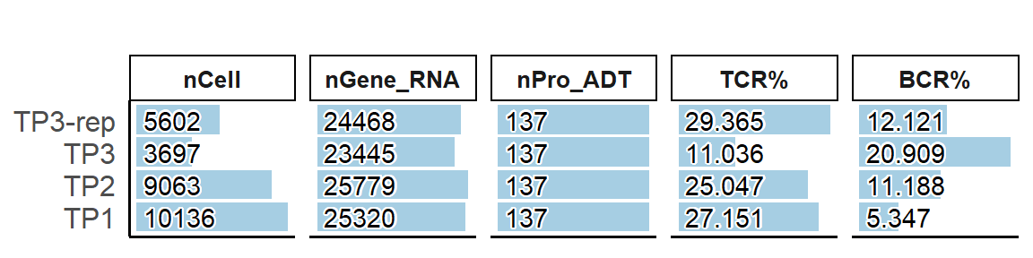
# Show sample metrics
ShowSampleMetricsName(pbmc, type = "summary")
##  [1] "nCount_RNA"            "nFeature_RNA"          "nCount_ADT"            "nFeature_ADT"          "percent.mt"            "percent.rb"
##  [7] "percent.hb"            "percent.dissociation"  "per_feature_count_RNA" "per_feature_count_ADT"
# Visualisation of summary of cell metrics.
PlotSampleMetrics(pbmc, type="summary", metrics=c("percent.mt"), return.type = "plot" )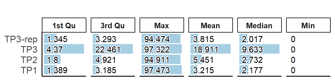
Visualising metrics using interactive table
When the information from the interactive table is displayed, the file can be saved in CSV format by clicking on the “Download as CSV” button in the top left hand corner. This is also possible with the following interactive tables.
# Show interactive table.
out<-PlotSampleMetrics(pbmc, type="summary", metrics=c("percent.mt"), return.type = "interactive_table" )
#Count information in the interaction table
out$baseMetrics
Metrics summary table
Visualising metrics using violin diagram
Violin plots can also be used to show metrics information between samples, only for cell metrics.
## Show cell metrics
ShowCellMetricsName(pbmc)
##  [1] "receptor_type"         "receptor_subtype"      "chain_pair"            "nChain_TRA"            "nChain_TRB"            "nChain_BCR"
##  [7] "nChain_IGH"            "nChain_IGK"            "nChain_IGL"            "orig.ident"            "nCount_RNA"            "nFeature_RNA"
## [13] "nCount_ADT"            "nFeature_ADT"          "percent.mt"            "percent.rb"            "percent.hb"            "percent.dissociation"
## [19] "per_feature_count_RNA" "per_feature_count_ADT" "percent.isotype"
# Select mitochondrial information to display by specifying ‘metrics’.
PlotCellMetrics(pbmc, group.by = "orig.ident", metrics = c("percent.mt"))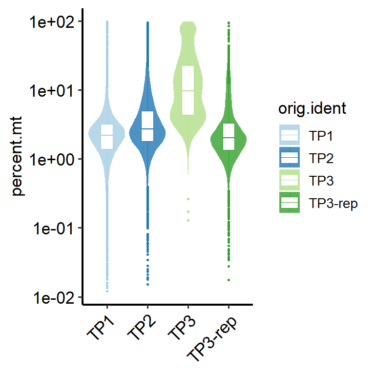
3.1.2.2 Using MAD to flag sample metrics warnings
To identify potential warning samples, SingleCellMQC employs the FindSampleMetricsWarning function, which applies Median Absolute Deviation (MAD) to flag samples deviating from general distributions of key QC metrics. By default, the metrics analyzed include: nCount_RNA, nFeature_RNA, nCount_ADT, nFeature_ADT, percent.mt, and percent.isotype.
out table
out <- FindSampleMetricsWarning(pbmc, sample.by = "orig.ident")
##   nCount_RNA warning samples: TP3
##   nFeature_RNA warning samples: TP3
##   nCount_ADT warning samples: TP2
##   percent.mt warning samples: TP3

# View the format of the table
str(out)
## List of 2
##  $ table:'data.frame':   24 obs. of  7 variables:
##   ..$ sample       : chr [1:24] "TP1" "TP2" "TP3" "TP3-rep" ...
##   ..$ metrics_name : chr [1:24] "nCount_RNA" "nCount_RNA" "nCount_RNA" "nCount_RNA" ...
##   ..$ metrics_value: num [1:24] 3990 3627 2079 4042 1680 ...
##   ..$ cutoff       : num [1:24] 2989 2989 2989 2989 1328 ...
##   ..$ type         : chr [1:24] "lower" "lower" "lower" "lower" ...
##   ..$ log          : logi [1:24] TRUE TRUE TRUE TRUE TRUE TRUE ...
##   ..$ isFlagged    : 'outlier.filter' logi [1:24] FALSE FALSE TRUE FALSE FALSE FALSE ...
##   .. ..- attr(*, "thresholds")= Named num [1:2] 2989 Inf
##   .. .. ..- attr(*, "names")= chr [1:2] "lower" "higher"
##  $ list :List of 6
##   ..$ nCount_RNA     : chr "TP3"
##   ..$ nFeature_RNA   : chr "TP3"
##   ..$ nCount_ADT     : chr "TP2"
##   ..$ nFeature_ADT   : chr(0)
##   ..$ percent.mt     : chr "TP3"
##   ..$ percent.isotype: chr(0)
interactive table
out <- FindSampleMetricsWarning(pbmc, sample.by = "orig.ident", return.type = "interactive_table")
##   nCount_RNA warning samples: TP3
##   nFeature_RNA warning samples: TP3
##   nCount_ADT warning samples: TP2
##   percent.mt warning samples: TP3
outMetrics warning results (MAD Statistics)
plot
out <- FindSampleMetricsWarning(pbmc, sample.by = "orig.ident", return.type = "plot")
##   nCount_RNA warning samples: TP3
##   nFeature_RNA warning samples: TP3
##   nCount_ADT warning samples: TP2
##   percent.mt warning samples: TP3
out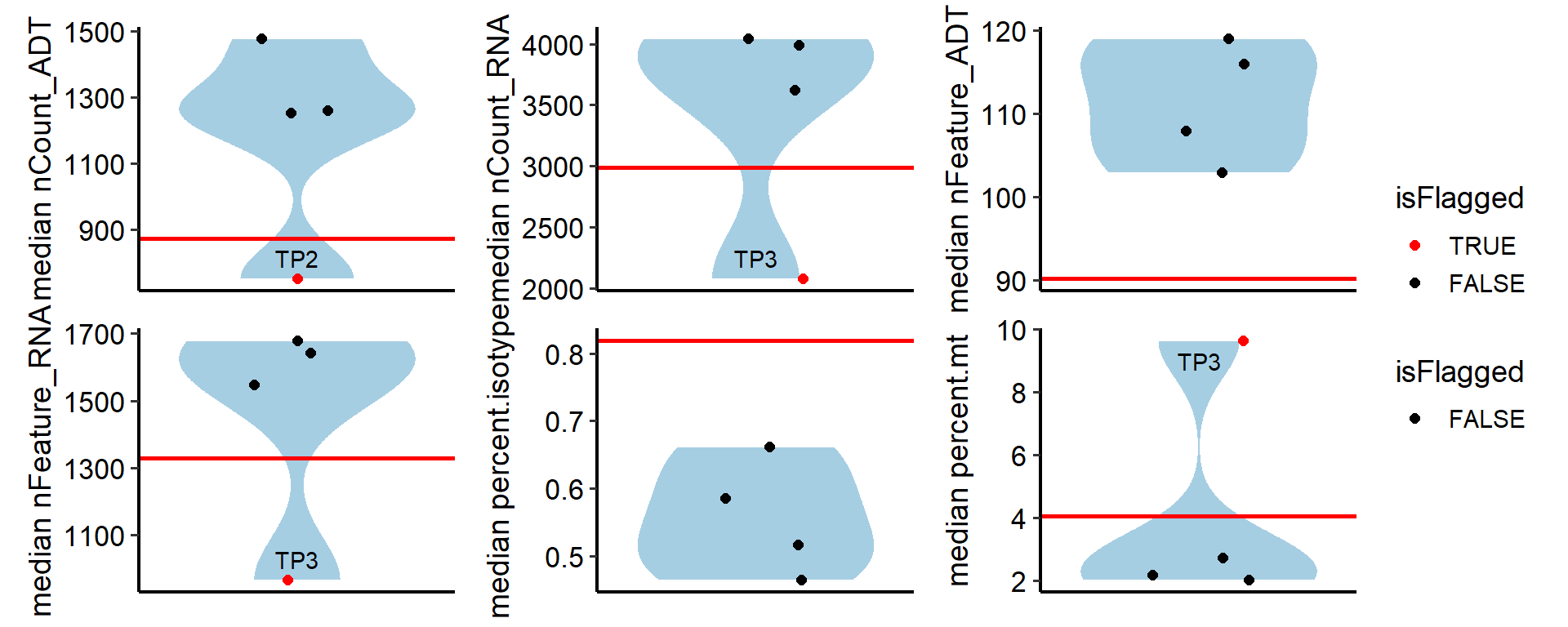
custom metrics
# Metrics of interest can be selected to output freely viewable interactive tables.
interactive_table <- FindSampleMetricsWarning(
  pbmc,
  metrics.by = c("nCount_RNA", "nFeature_RNA", "nCount_ADT", "nFeature_ADT",
                 "percent.mt", "percent.isotype", "TCR%"),
  type = c("lower", "lower", "lower", "lower", "higher", "higher", "lower"),
  log = c(TRUE, TRUE, TRUE, TRUE, FALSE, FALSE, FALSE),
  nmads = c(3, 3, 3, 3, 3, 3, 3),
  return.type = "interactive_table"
)
##   nCount_RNA warning samples: TP3
##   nFeature_RNA warning samples: TP3
##   nCount_ADT warning samples: TP2
##   percent.mt warning samples: TP3
##   TCR% warning samples: TP3
interactive_tableMetrics warning results (MAD Statistics)
3.1.3 Visualisation of V(D)J data
pct: for the percentage of chain type
The input object must be a Seurat object containing V(D)J information, which can be obtained using the ‘CalculateMetrics’ function.
# Demonstration of anomalies in the V(D)J data
# When viewing the results, it is necessary to display them in a second level, e.g. ‘plot_list$TCR’.
plot_list <- PlotSampleVDJ(pbmc, type="pct", return.type = "plot")
## > - 0 TRA% > TRB% samples, 4 TRA% <= TRB% samples.
## > - 0 IGH% > (IGK+IGL)% samples, 4 IGH% <= (IGK+IGL)% samples.
## > - 1 BCR% > TCR% samples : `TP3`
names(plot_list)
## [1] "TCR" "BCR" "VDJ"
plot_list$VDJ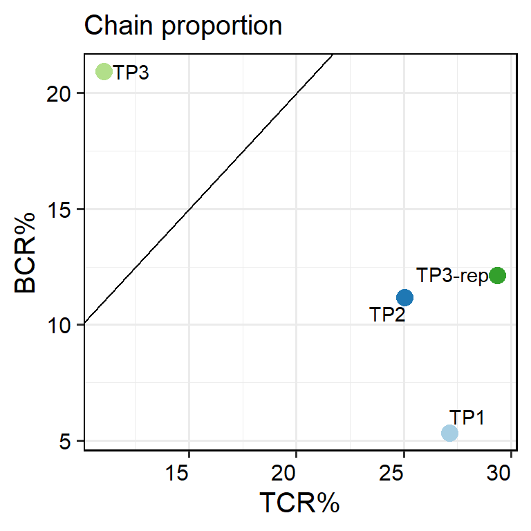
# interactive table
out <- PlotSampleVDJ(pbmc, type="pct", return.type = "interactive_table")
## > - 0 TRA% > TRB% samples, 4 TRA% <= TRB% samples.
## > - 0 IGH% > (IGK+IGL)% samples, 4 IGH% <= (IGK+IGL)% samples.
## > - 1 BCR% > TCR% samples : `TP3`
# out$base stores the sample base information for the V(D)J chain.
out$baseV(D)J chain
V(D)J chain summary table
subtype: for the percentage of chain subtype
The input object must be a Seurat object containing V(D)J information, which can be obtained using the ‘CalculateMetrics’ function.
# Distribution of receptor subtype occupancy among samples
out<-PlotSampleVDJ(pbmc, type="subtype", return.type = "plot")
out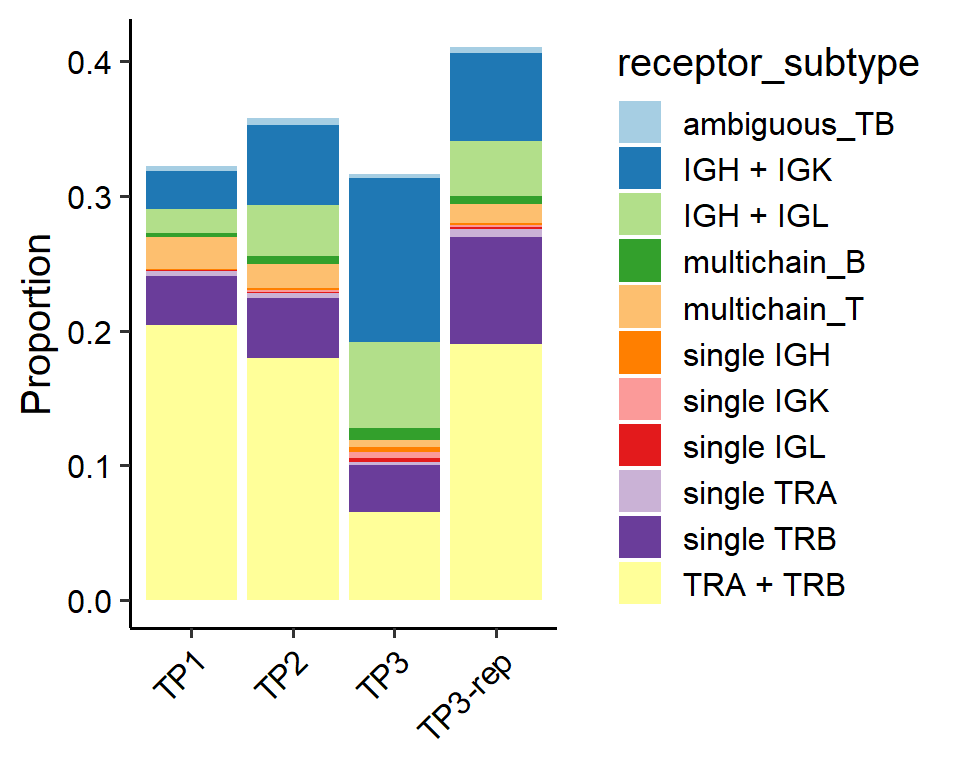
# interactive table
out <- PlotSampleVDJ(pbmc, type="subtype", return.type = "interactive_table")
# out$base stores information about the receptor subtypes of the V(D)J data
out$baseVDJ subtype
VDJ subtype summary table
If the
typeparameter is set to “CDR3”, “clonalQuant”, “clonalOverlap”, or “geneUsage”, the input must be a list generated by theRead10XDatafunction and preprocessed using the scRepertoire package.
# Reading of V(D)J data
dir_TCR <- c(
"/data/SingleCellMQC/CellRanger/TP1/vdj_t/filtered_contig_annotations.csv",
"/data/SingleCellMQC/CellRanger/TP2/vdj_t/filtered_contig_annotations.csv",
"/data/SingleCellMQC/CellRanger/TP3/vdj_t/filtered_contig_annotations.csv",
"/data/SingleCellMQC/CellRanger/TP3-rep/vdj_t/filtered_contig_annotations.csv"
)
sample_name <- c("TP1", "TP2", "TP3", "TP3-rep")
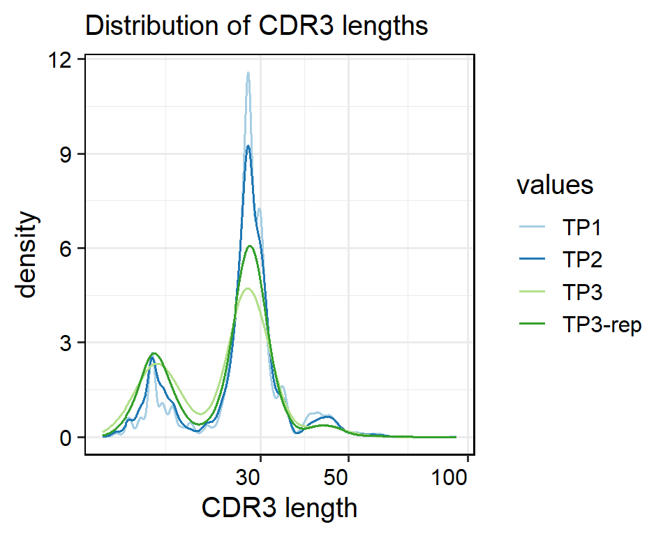
VDJ_data <- Read10XData(dir_TCR = dir_TCR, sample = sample_name)CDR3: for the length distribution of the CDR3 sequences
The input object must be a raw list of “filtered_contig_annotations” data as input, details see clonalLength function from scRepertoire package.
clonalQuant: or quantifying unique clonotypes
The input object must be a raw list of “filtered_contig_annotations” data as input, details see clonalQuant function from scRepertoire package.
# CDR3 length visualisation
out<-PlotSampleVDJ(VDJ_data, type="clonalQuant", return.type = "plot")
out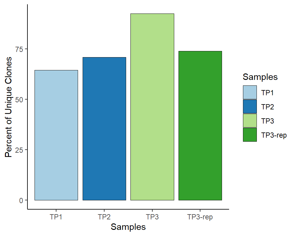
clonalOverlap: for quantifying unique clonotypes
The input object must be a raw list of “filtered_contig_annotations” data as input, details see clonalOverlap function from scRepertoire package.
# clonalOverlap visualisation
out<-PlotSampleVDJ(VDJ_data, type="clonalOverlap", return.type = "plot")
out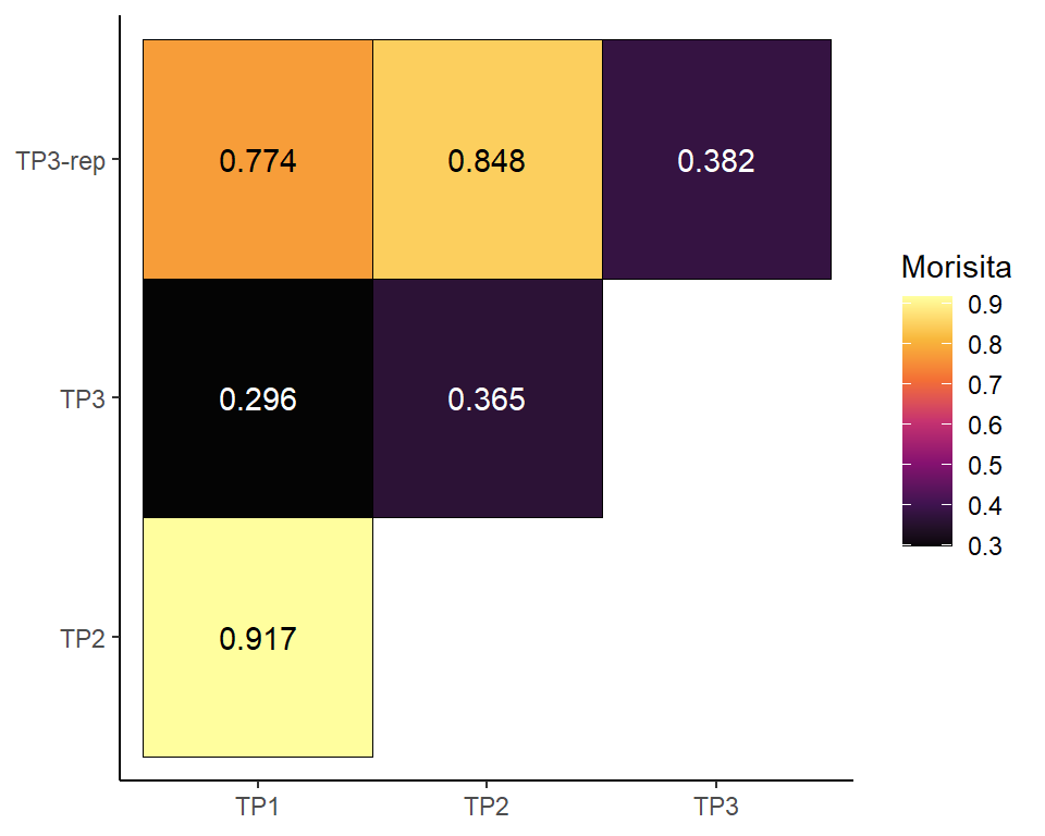
# interactive table
out <- PlotSampleVDJ(VDJ_data, type="clonalOverlap", return.type = "interactive_table")
outMorisita
geneUsage: for the proportion of V gene usage
The input object must be a raw list of “filtered_contig_annotations” data as input, details see percentGenes function from scRepertoire package.
# GeneUsage visualisation
PlotSampleVDJ(VDJ_data, type="geneUsage", return.type = "plot")
# interactive_table
out <- PlotSampleVDJ(VDJ_data, type="geneUsage", return.type = "interactive_table")
out geneUsage
3.2 PCT outlier sample detection
Outlier sample detection in SingleCellMQC focuses on identifying deviations in cell type composition. Deviations in cell type composition within samples from the same experimental group are often indicative of potential technical issues, such as prolonged processing time, variations in storage conditions, experimental processing errors, and batch effects, all of which can compromise the integrity of the data. To address this issue, SingleCellMQC incorporates cell type composition analysis as a additional outlier detection approach. This section include two main approaches: 1) Common range outliers: Comparison of predicted results with cell proportion range database; 2) Inter-sample outliers: Identifying deviations in cell type composition.
3.2.1 Cell type annotation (ScType)
The data needs to be performed automatic cell annotation, selecting either the “Main” or “ScType” or “Cell_Taxonomy” database for annotation in RunScType(). The “Main” database is annotated by default and contains T cells, B cells, NK cells, DC cells, Mon / Mac cells, endothelial cells, fibroblasts, granulocytes and other cells (erythrocytes, epithelial cells, etc.).
# To view the types of organisations included in the Cell_Taxonomy database
head(ShowDatabaseTissue(database="Cell_Taxonomy"))
## [1] "Brain"          "Embryo"         "Ovary"          "Prostate gland" NA               "Blood"
# To view the types of organisations included in the ScType database
head(ShowDatabaseTissue(database = "ScType"))
## [1] "Immune system" "Pancreas"      "Liver"         "Eye"           "Kidney"        "Brain"
# For each sample, the cells were annotated separately.
pbmc <- RunScType(pbmc, split.by="orig.ident", data_source = "Main")
# The results are stored in the ScType column of meta.data
table(pbmc@meta.data$ScType)##
## B cell DC Mon/Mac NK Other T cell
## 3436 460 5653 5059 2522 113683.2.2 Comparison of predicted results with cell proportion range database
This section provides a summary of the common range outliers based on cell type composition. Outlier samples can be identified by comparing their cell type composition with our established reference cell type composition ranges when performing the FindCommonPCTOutlier function. The reference cell type composition ranges are established based on the 2299 single cell samples from DISCO database.
FindCommonPCTOutlier() can be used to determine if the sample is out of scale with the database and output the outlier sample. Currently only auto-annotated results from the Main database are supported.
FindCommonPCTOutlier(pbmc, tissue = "blood", return.type = "interactive_table", celltype.by = "ScType")
##   T cell outlier samples: TP3
##   B cell outlier samples: TP3
## Other outlier samples: TP2,TP3Common range outlier results
3.2.3 Inter-sample outliers
A PCA-based outlier detection method using confidence ellipse or Density-Based Spatial Clustering of Applications with Noise (DBSCAN) to identify samples with unusual cell type proportions within sample groups was also provided in this section. Additionally, contributions of each cell type composition to PCs were calculated, providing further insights into potential outliers and ensuring the reliability of the dataset for downstream analysis.
Flag samples with unusual proportions of cell types within sample groups:confidence ellipse
# Identify outliers using the confidence ellipse

# Use return.type to specify the type of output, including table, plot and interactive table
out <- FindInterSamplePCTOutlier(pbmc, method = "ellipse", confidence_level = 0.95, return.type = "plot")
## Outlier samples:
# PCA plot
out$pca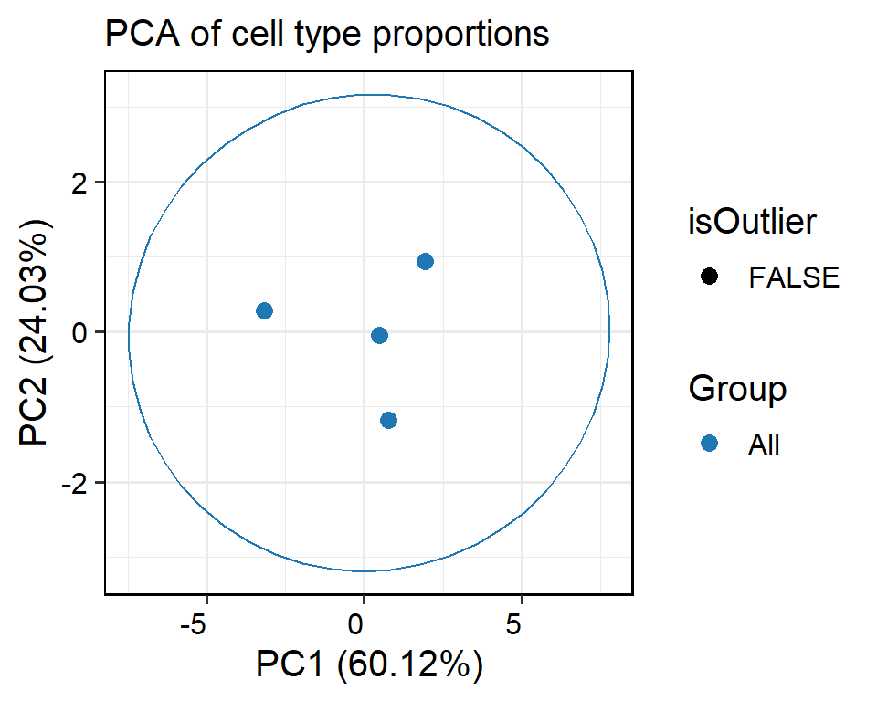
DBSCAN
out <- FindInterSamplePCTOutlier(pbmc, method = "dbscan",  return.type = "plot")
## Outlier samples: TP3
# PCA plot
out$pca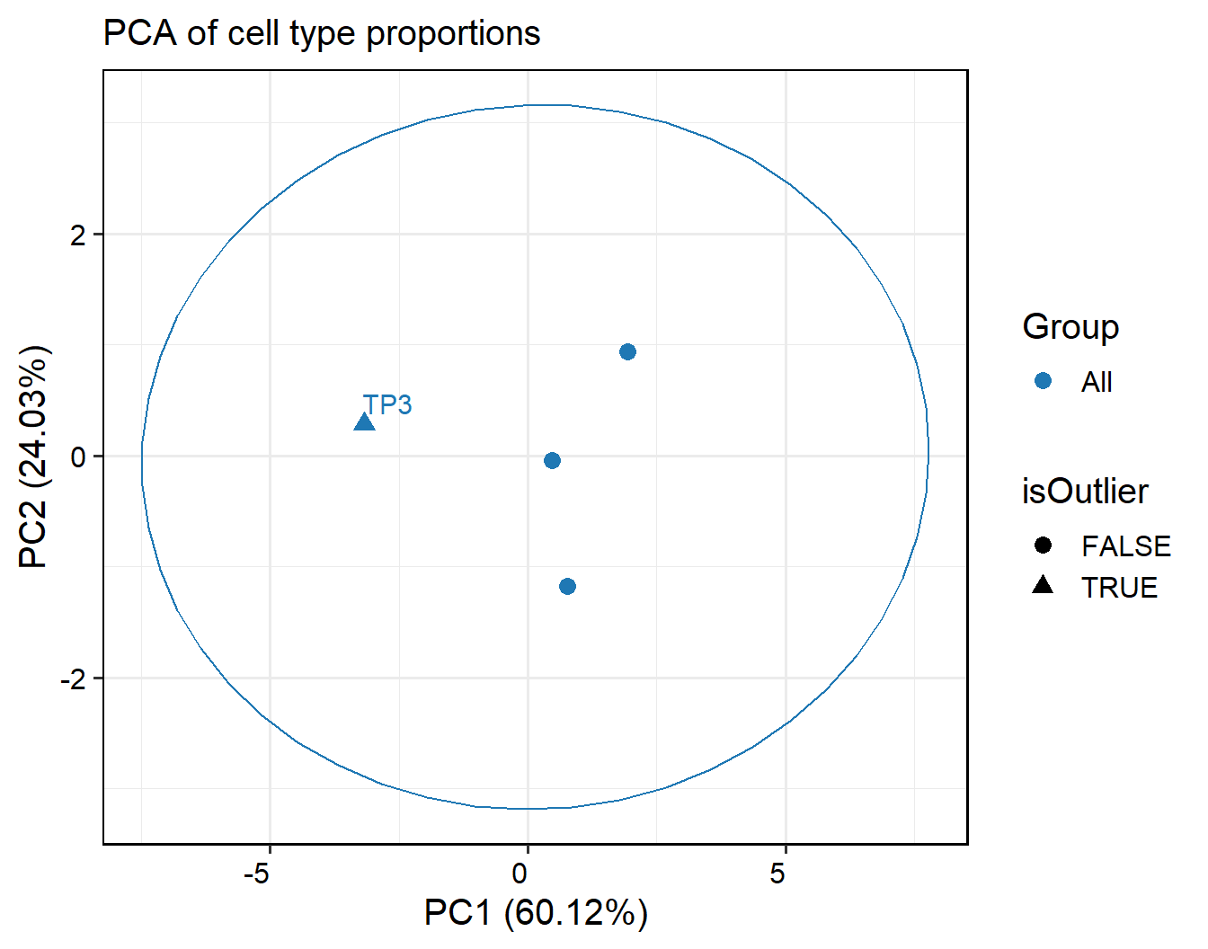
# interactive table
out <- FindInterSamplePCTOutlier(pbmc, celltype.by = "ScType", sample.by = "orig.ident", return.type="interactive_table")
## Outlier samples:
# Cell PCT Outlier results are shown in the out$outlier.
out$outlierCell PCT Outlier results
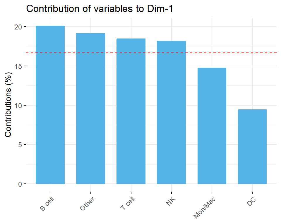
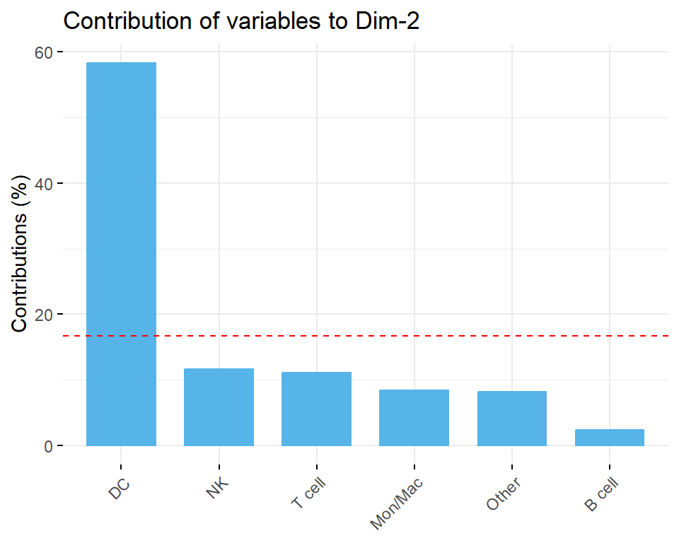
Contribution of groups to PCs
3.2.4 Outlier detection for metrics with different cell types
# Visualisation of the results
outlier_result <- FindSampleMetricsWarning(pbmc, split.by="ScType",
                                                sample.by = "orig.ident",return.type="plot")
## >>>>>> B cell
##   nCount_ADT warning samples: TP2
##   percent.mt warning samples: TP3
## >>>>>> DC
##   percent.mt warning samples: TP3
## >>>>>> Mon/Mac
##   nFeature_RNA warning samples: TP3
##   percent.mt warning samples: TP3
##   percent.isotype warning samples: TP3
## >>>>>> NK
##   percent.mt warning samples: TP3
## >>>>>> Other
##   nFeature_ADT warning samples: TP2
## >>>>>> T cell
##   nCount_ADT warning samples: TP2
##   percent.mt warning samples: TP3
# The metrics of interest can be selected to be displayed
outlier_result[["T cell"]]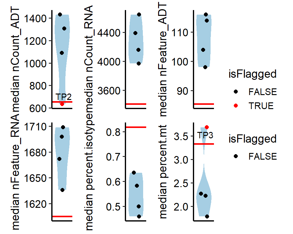
# interactive table
outlier_result <- FindSampleMetricsWarning(pbmc, split.by="ScType",
                                           sample.by = "orig.ident",return.type="interactive_table")
## >>>>>> B cell
##   nCount_ADT warning samples: TP2
##   percent.mt warning samples: TP3
## >>>>>> DC
##   percent.mt warning samples: TP3
## >>>>>> Mon/Mac
##   nFeature_RNA warning samples: TP3
##   percent.mt warning samples: TP3
##   percent.isotype warning samples: TP3
## >>>>>> NK
##   percent.mt warning samples: TP3
## >>>>>> Other
##   nFeature_ADT warning samples: TP2
## >>>>>> T cell
##   nCount_ADT warning samples: TP2
##   percent.mt warning samples: TP3
# The metrics of interest can be selected to be displayed
outlier_resultMetrics outlier results (MAD Statistics)
3.2.5 Visualisation of the PCT of cell types
Based on the results of the automatic cell annotation, visualisation of cell proportions can be performed, including stacked plots, histograms and interaction tables.
# Stacked Bar Chart for all cell types
PlotSampleCellTypePCT(pbmc, sample.by = "orig.ident", celltype.by = "ScType", plot.type="stackbar")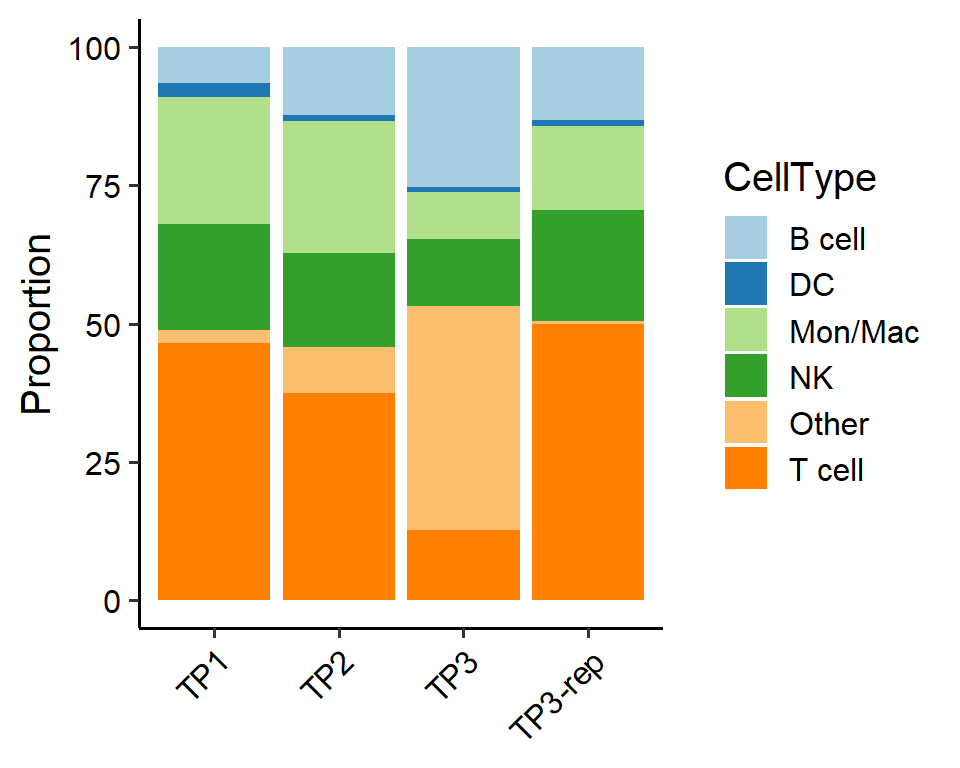
# Bar graphs for each cell type
PlotSampleCellTypePCT(pbmc, sample.by = "orig.ident", celltype.by = "ScType", plot.type = "bar")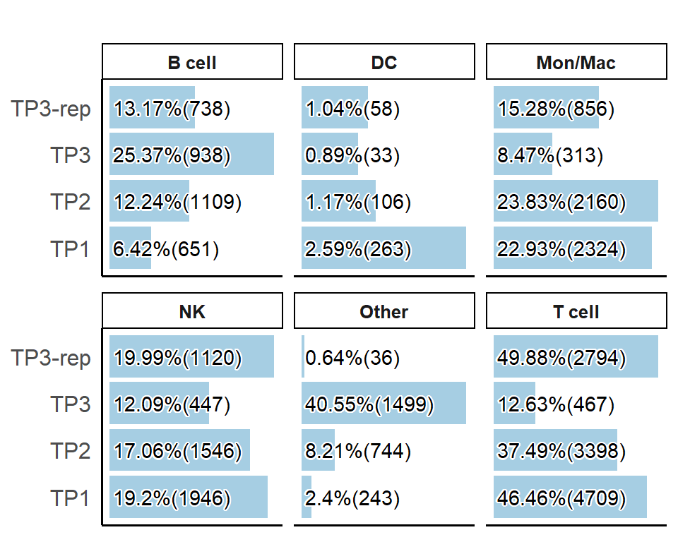
# interactive table
PlotSampleCellTypePCT(pbmc, sample.by = "orig.ident", celltype.by = "ScType", return.type="interactive_table")CellType% per Sample
3.3 Sample identity verification
To avoid potential recording mistakes and data transmission errors, checking whether the file labeling is consistent with analyzed data features is necessary at the beginning of sample QC. By default, you can check if your sample gender information is incorrectly labeled. In addition, if your sample does not have gender information, you can get it according to the table below. Use PlotSampleLabel() to visualise the percentage of gene expression, with gender-related genes set as the default.
The pct of features
It is possible to customise the gender-related genes to be analysed, e.g. “Female=‘XIST’, Male=c(‘DDX3Y’, ‘UTY’)”,store them with the “feature_list”.