4 Cell QC
Compiled: 2025-05-08 Written by Jiaying Zeng and Daihan Ji
library(SingleCellMQC)
#Load a pre-existing Seurat object or process raw data using SingleCellMQC.
pbmc <- readRDS("/data/pbmc.rds")
The cell-level QC in SingleCellMQC includes the identification of (i) empty droplets, (ii) doublets, and (iii) low-quality cells. By integrating a variety of publicly available tools and in-house developed QC strategies, the cell QC module provides a systematic framework to detect and remove problematic droplets or cells across multiple omics layers.
Where can you view the results of cell-level QC?
You can explore them in pbmc@meta.data or pbmc@misc[["SingleCellMQC"]][["perQCMetrics"]][[perCell]],pbmc@misc[["SingleCellMQC"]][["LowQuality"]],pbmc@misc[["SingleCellMQC"]][["Doublet"]].
4.1 Empty droplets detection (If Required)
Generally, count matrix files generated from single-cell preprocessing tools such as Cell Ranger and dnbc4tools have already undergone empty droplet removal. However, if users wish to perform this step themselves, SingleCellMQC implements empty droplet detection based on scRNA-seq data using the dropletUtils package.
4.2 Low quality cells detection
Before you conduct low quality cells detection, ensure that you have run CalculateMetrics.
4.2.1 Fixed cutoff
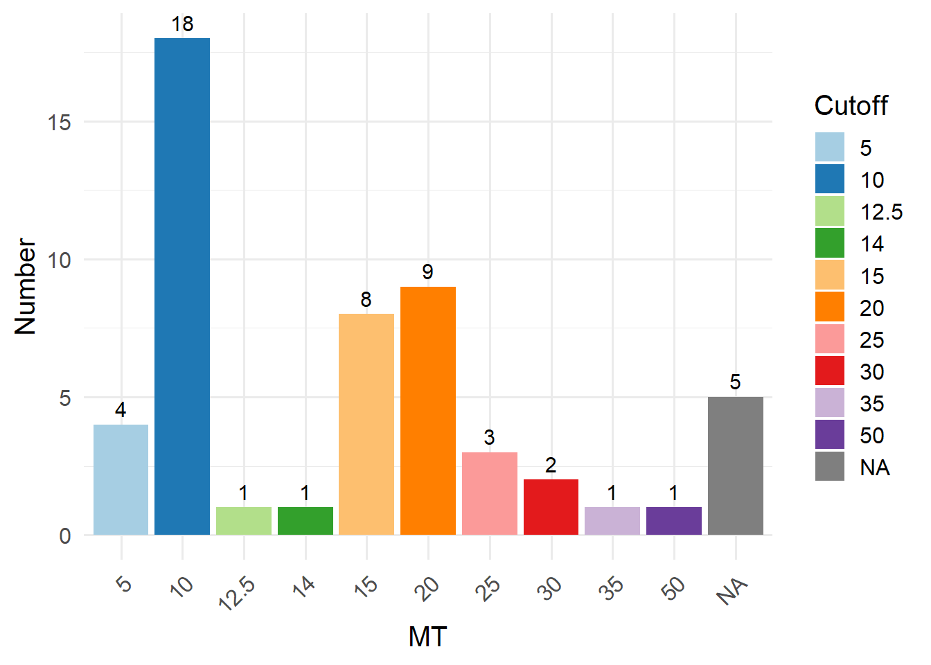
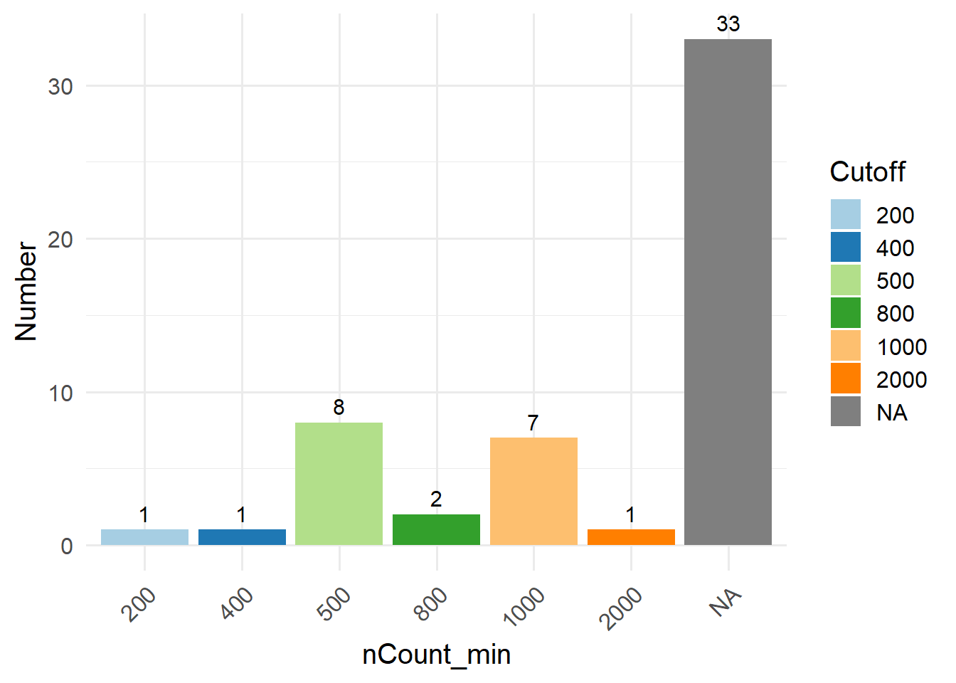
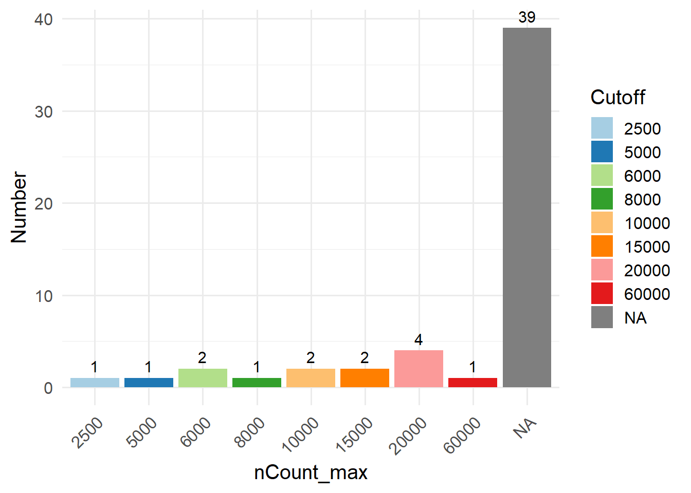
In this method, you can filter out low-quality cells by setting a fixed cutoff for certain cell QC metrics. Before choosing a suitable cutoff, you can use GetMetricsRange to obtain the commonly used cutoff for the corresponding tissue. The cutoffs for each QC parameter was obtained by 240 single-cell studies spanning 11 human tissues. Here, we take “blood” as an example.
Alternatively, you can visualize cell QC metrics using regular violin plots, and manually select appropriate cutoffs by yourself.
# View the cell QC metrics, such as percentage of mitochondria.
PlotCellMetrics(pbmc, metrics ="percent.mt" , log.y = F )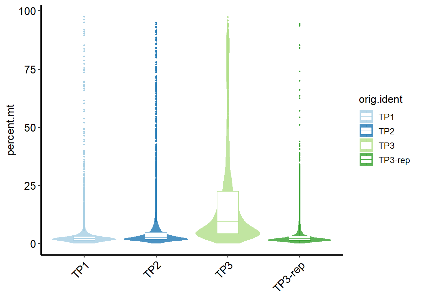
Then you can select your cutoff to set a fixed threshold to mark low-quality cells.
4.2.2 MAD method
You can use SingleCellMQC to automatically identify low-quality cells by calculating outliers for RNA metrics (nCount_RNA, nFeature_RNA, percent.mt) and ADT metrics (nCount_ADT, nFeature_ADT, percent.isotype) using the Median Absolute Deviation (MAD) method.
4.2.3 miQC method
Other publicly available tools for low-quality cells detection are integrated in this part. The miQC method is one of them. You can turn to reference and github link for more detailed information.
4.2.4 ddqc method
The ddqc method is another publicly available tool. You can turn to reference and github link for more detailed information.
4.3 Check low-quality cells (optional)
To minimize false positives, SingleCellMQC allows re-clustering of flagged cells based on their expression profiles before removal. This step helps identify biologically relevant cell populations that may exhibit outlier QC metrics due to molecular expression variability rather than poor quality, and these cells are rescued and retained for downstream analysis.
# pbmc <- RunLQ_fixed(pbmc, min.nFeature_RNA = 200, min.nCount_RNA = 500, percent.mt = 10)
# For `method_column` parameter, enter the colnames of the result of previous methods that you want to re-cluster, such as "lq_Fixed".
out <- RunLQReClustering(pbmc, method_column = c("lq_fixed"),cluster_resolution = 1)
After the re-clustering is completed, the following three parts can be used to confirm the cell identity and check whether there are any missed cell groups.
- Use
COSGmethod to find markers in each low-quality cluster, assisting in cell identity determination.
##        gene cluster  cosg avg_logFC meanlog_1 meanlog_2  pct_1  pct_2
## GNLY   GNLY  Fail_4 0.321     1.826    3.1322    1.3065 0.6639 0.1033
## MATK   MATK  Fail_4 0.219     1.028    1.2990    0.2708 0.2389 0.0384
## SPON2 SPON2  Fail_4 0.198     1.202    1.7013    0.4992 0.3444 0.0621
## SYNE1 SYNE1  Fail_4 0.197     1.177    2.1275    0.9501 0.5333 0.1491
## CCL5   CCL5  Fail_4 0.187     1.301    2.7265    1.4259 0.6583 0.1589
## SYTL2 SYTL2 Fail_4 0.182 0.956 1.3290 0.3731 0.2500 0.0504- Call
ClusterProfilerpackage to perform pathway enrichment analysis to view the pathways of each low-quality cluster, assisting in cell identity determination.
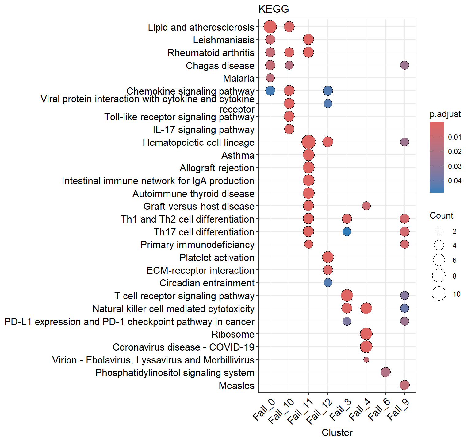
- Perform
ScTypeannotation to assist in determining cell identities. Cells labeled as “Unknown” are more likely to represent low-quality cells.
LQ_result <- RunScType(LQ_result, data_source ="ScType")
PlotReducedDim(LQ_result, group.by = "seurat_clusters")+
PlotReducedDim(LQ_result, group.by = "ScType")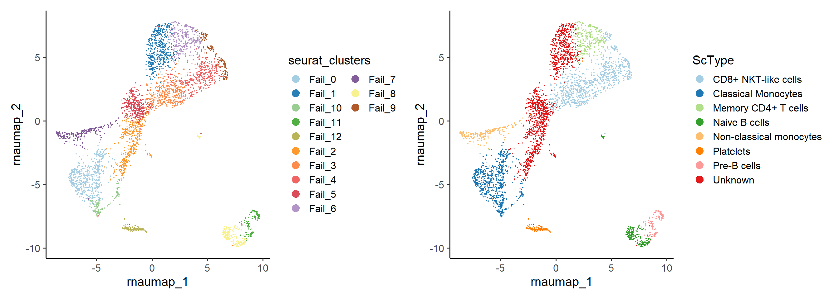
4.4 Doublets detection
For doublets detection, SingleCellMQC integrates five widely used RNA expression-based methods, including DoubletFinder, scDbFinder, cxds, bcds, hybrid, one V(D)J chain based method on TCR/BCR sequencing data, along with one in-house developed multi-omics strategy based on surface protein expression (ADT-based).
4.4.1 scDblFinder method
The scDblFinder method is one of the publicly available tools for doublets detection. You can turn to reference and github link for more detailed information.
# The `split.by` parameter must refer to your sample.
# The `add.Seurat` parameter means whether you want to add results in the Seurat object.
pbmc<- RunDbt_scDblFinder(pbmc, split.by = "orig.ident", add.Seurat=T, do.topscore=T)table(pbmc$db_scDblFinder, pbmc$orig.ident)
##
## TP1 TP2 TP3 TP3-rep
## Fail 821 657 109 251
## Pass 9315 8406 3588 5351
head(pbmc$db_scDblFinder_score)
## TP1_AAACCTGAGAATGTTG-1 TP1_AAACCTGAGCCCTAAT-1 TP1_AAACCTGAGGACTGGT-1 TP1_AAACCTGCAAGCGATG-1 TP1_AAACCTGCAATGGAGC-1 TP1_AAACCTGCACAGTCGC-1
## 0.0060459864 0.9996028543 0.0016912580 0.0008436530 0.9318320155 0.00011877444.4.2 hybrid method
The hybrid method is one of the publicly available tools for doublets detection. You can turn to reference and github link for more detailed information.
# The `split.by` parameter must refer to your sample.
# The `add.Seurat` parameter means whether you want to add results in the Seurat object.
pbmc<- RunDbt_hybrid(pbmc, split.by = "orig.ident", add.Seurat=T)table(pbmc$db_hybrid, pbmc$orig.ident)
##
## TP1 TP2 TP3 TP3-rep
## Fail 821 657 109 251
## Pass 9315 8406 3588 5351
head(pbmc$db_hybrid_score)
## TP1_AAACCTGAGAATGTTG-1 TP1_AAACCTGAGCCCTAAT-1 TP1_AAACCTGAGGACTGGT-1 TP1_AAACCTGCAAGCGATG-1 TP1_AAACCTGCAATGGAGC-1 TP1_AAACCTGCACAGTCGC-1
## 0.3104272 1.7186222 0.2577161 0.2417090 1.0813173 0.08432164.4.3 bcds method
The bcds method is one of the publicly available tools for doublets detection. You can turn to reference and github link for more detailed information.
# The `split.by` parameter must refer to your sample.
# The `add.Seurat` parameter means whether you want to add results in the Seurat object.
pbmc<- RunDbt_bcds(pbmc, split.by = "orig.ident", add.Seurat=T)table(pbmc$db_bcds, pbmc$orig.ident)
##
## TP1 TP2 TP3 TP3-rep
## Fail 821 657 109 251
## Pass 9315 8406 3588 5351
head(pbmc$db_bcds_score)
## TP1_AAACCTGAGAATGTTG-1 TP1_AAACCTGAGCCCTAAT-1 TP1_AAACCTGAGGACTGGT-1 TP1_AAACCTGCAAGCGATG-1 TP1_AAACCTGCAATGGAGC-1 TP1_AAACCTGCACAGTCGC-1
## 0.01293355 0.93673164 0.02887737 0.02212005 0.80253756 0.016730224.4.4 cxds method
The cxds method is one of the publicly available tools for doublets detection. You can turn to reference and github link for more detailed information.
# The `split.by` parameter must refer to your sample.
# The `add.Seurat` parameter means whether you want to add results in the Seurat object.
pbmc<- RunDbt_cxds(pbmc, split.by = "orig.ident", add.Seurat=T)table(pbmc$db_cxds, pbmc$orig.ident)
##
## TP1 TP2 TP3 TP3-rep
## Fail 821 657 109 251
## Pass 9315 8406 3588 5351
head(pbmc$db_cxds_score)
## TP1_AAACCTGAGAATGTTG-1 TP1_AAACCTGAGCCCTAAT-1 TP1_AAACCTGAGGACTGGT-1 TP1_AAACCTGCAAGCGATG-1 TP1_AAACCTGCAATGGAGC-1 TP1_AAACCTGCACAGTCGC-1
## 160102.42 497734.06 147398.61 145724.55 212804.72 46557.394.4.5 DoubletFinder method
The DoubletFinder method is one of the publicly available tools for doublets detection. You can turn to reference and github link for more detailed information.
# The `split.by` parameter must refer to your sample.
# The `add.Seurat` parameter means whether you want to add results in the Seurat object.
pbmc<- RunDbt_DoubletFinder(pbmc, split.by = "orig.ident", add.Seurat=T)table(pbmc$db_DoubletFinder, pbmc$orig.ident)
##
## TP1 TP2 TP3 TP3-rep
## Fail 821 657 109 251
## Pass 9315 8406 3588 5351
head(pbmc$db_DoubletFinder_score)
## TP1_AAACCTGAGAATGTTG-1 TP1_AAACCTGAGCCCTAAT-1 TP1_AAACCTGAGGACTGGT-1 TP1_AAACCTGCAAGCGATG-1 TP1_AAACCTGCAATGGAGC-1 TP1_AAACCTGCACAGTCGC-1
## 0.1684285 0.3484848 0.1758280 0.1370684 0.2152925 0.20260754.4.6 VDJ method
The VDJ-based strategy can identify homotypic doublets by detecting multi-chain cells. In immune repertoire sequencing, cells with multiple TCR or BCR chains (or both) are flagged as potential doublets.
4.4.7 ADT method
The ADT-based strategy can identify heterotypic doublets by analyzing mutually exclusive surface markers in ADT sequencing. This ADT-based method calculates positive expression thresholds for each surface protein. Cells with both expressions of exclusive paired surface markers were considered as doublets (Details see our manuscript). Users can customize exclusive surface marker pairs to target specific cell types based on their experiment needs, such as CD19 and CD3, which differentiate B and T cells. Here we take CD20/CD3 and CD19/CD3 as examples.
You can use the ADT method to detect doublets. In default mode, ADT-based clustering is applied.
pbmc <- RunDbt_ADT(pbmc, split.by = "orig.ident", add.Seurat =T,
                   feature1 = c("Hu.CD20-2H7","Hu.CD19"),
feature2 = c("Hu.CD3-UCHT1","Hu.CD3-UCHT1"))table(pbmc$db_ADT, pbmc$orig.ident)
##
## TP1 TP2 TP3 TP3-rep
## Fail 87 165 153 75
## Pass 10049 8898 3544 5527
If you are concerned about the impact of protein background noise, you can use the do.correct parameter to call the scCDC package to denoise the ADT data.
What if you want to return the threshold of expression levels used to distinguish between negative and positive cell populations?
# Calculate the cutoff of doublets
cutoff <- RunDbt_ADT(pbmc, feature1 = c("Hu.CD20-2H7","Hu.CD19"),
                   feature2 = c("Hu.CD3-UCHT1","Hu.CD3-UCHT1"),
return.cutoff = T, split.by = "orig.ident")head(cutoff)
## Sample cluster_num resolution feature1 cutoff1 feature2 cutoff2
## 1 TP1 24 1.5 Hu.CD20-2H7 0.7860469 Hu.CD3-UCHT1 1.178921
## 2 TP1 24 1.5 Hu.CD19 0.7283664 Hu.CD3-UCHT1 1.178921
## 3 TP2 24 1.5 Hu.CD20-2H7 0.8705569 Hu.CD3-UCHT1 1.029872
## 4 TP2 24 1.5 Hu.CD19 0.5773097 Hu.CD3-UCHT1 1.029872
## 5 TP3 21 1.5 Hu.CD20-2H7 0.8418260 Hu.CD3-UCHT1 1.227219
## 6 TP3 21 1.5 Hu.CD19 0.5099738 Hu.CD3-UCHT1 1.227219
# Check out the results of TP1
PlotADTCutoff(pbmc, cutoff, feature1 = "Hu.CD20-2H7", feature2 = "Hu.CD3-UCHT1",
Sample="TP1", group.by = "chain_pair")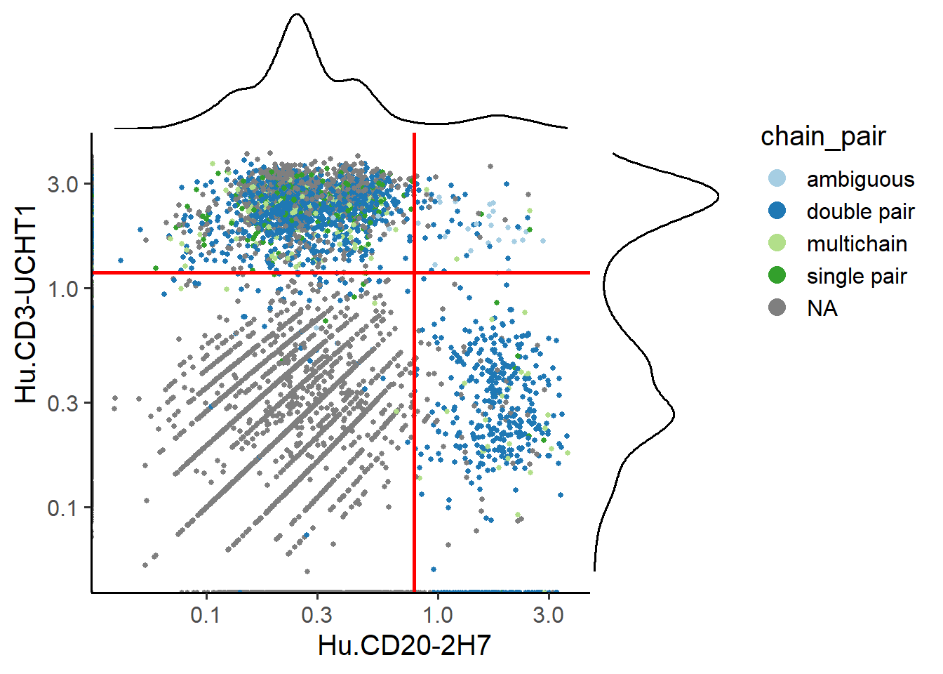
4.5 Visualization of cell QC results
4.5.1 Visualization of the percentage of cells filtered by different methods
# Choose the detection session you want in `type.detection` parameter, including "lq" for low-quality cells and "db" for doublets.
# Plotting the percentage of cells filtered by low-quality cell detection methods
PlotCellMethodFiltration(pbmc, type.detection = "lq", return.type = "plot")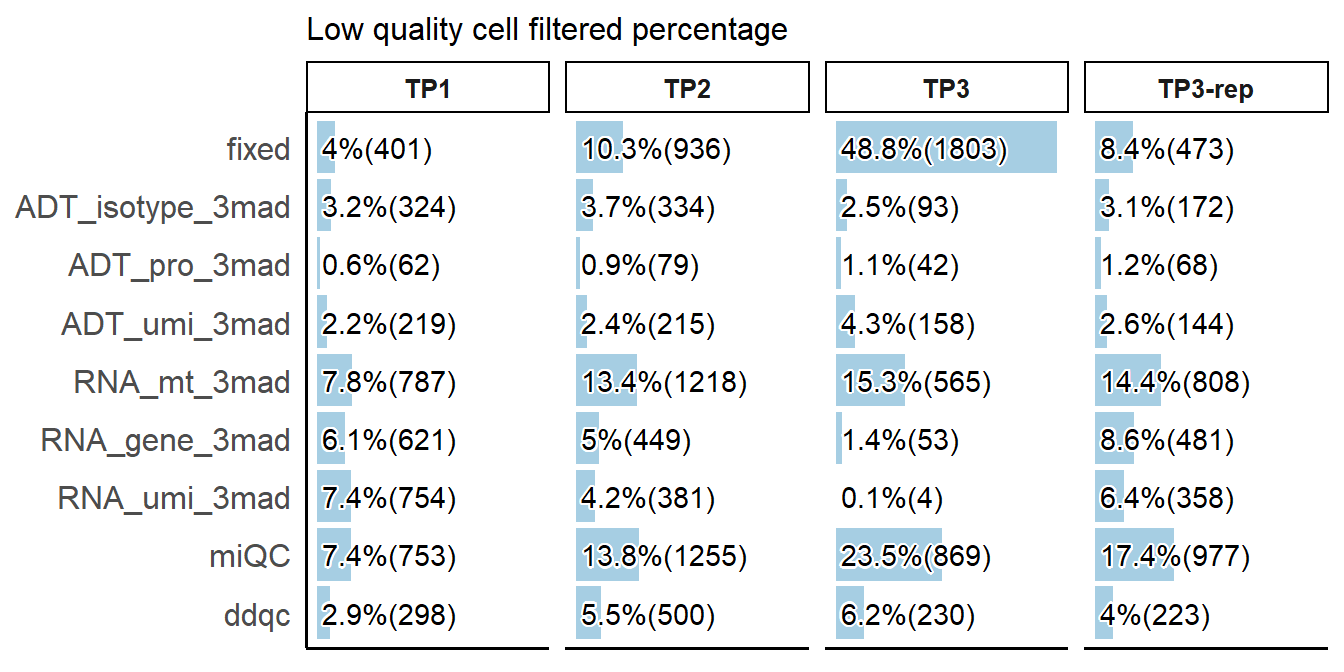
# Plotting the percentage of cells filtered by doublet detection methods
PlotCellMethodFiltration(pbmc, type.detection = "db", return.type = "plot")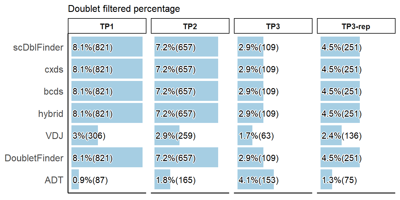
# Plotting interactive table
interactive_table <- PlotCellMethodFiltration(pbmc, type.detection = "lq", return.type = "interactive_table")
interactive_table$pct ##Show filtered percentagesLow quality cell filtered percentage
Low quality cell filtered number
4.5.2 Overlap between different methods (UpSet plot)
Low-quality cell results as an example, the same applies to doublet methods.
# Plotting overlap of low-quality cell detection methods (all samples).
PlotCellMethodUpset(pbmc, type.detection = "lq")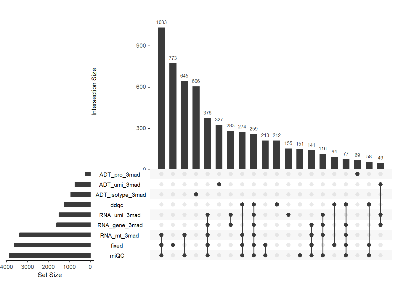
# Plotting overlap of low-quality cell detection methods (each sample).
# Choose the column representing your sample for the `split.by` parameter.
out <- PlotCellMethodUpset(pbmc, type.detection = "lq", split.by = "orig.ident")
names(out)
## [1] "TP1" "TP2" "TP3" "TP3-rep"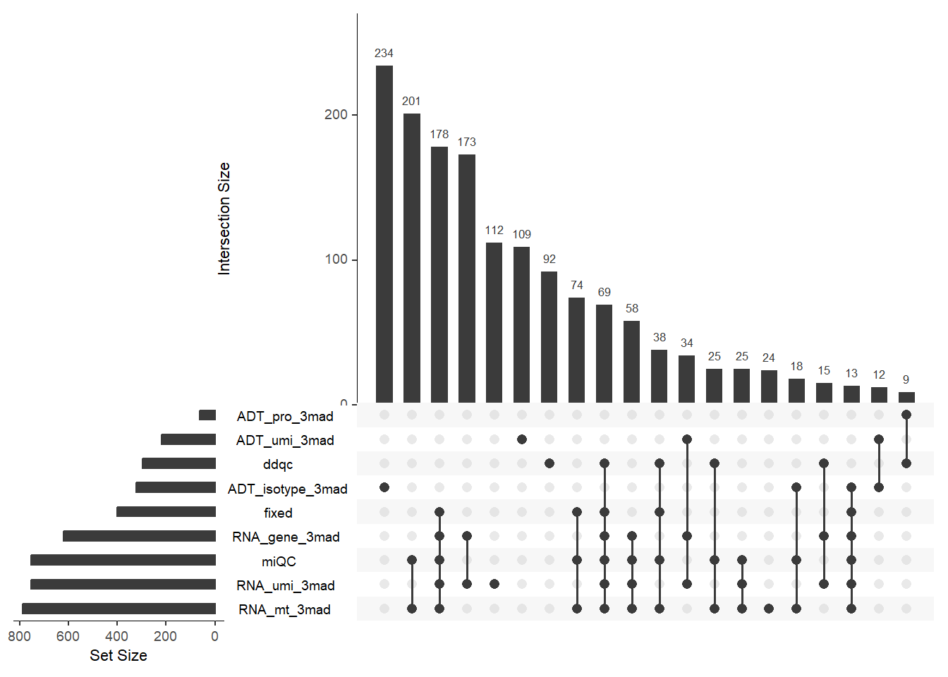
4.5.3 Comparison of metrics between Pass and Fail cells identified by methods
Taking percentage of percent.mt of low-quality cells as an example, the same applies to other metrics and doublets.
# Plotting comparison of low-quality cell detection methods (all samples).
PlotCellMethodVln(pbmc, metrics.by = "percent.mt", type.detection = "lq")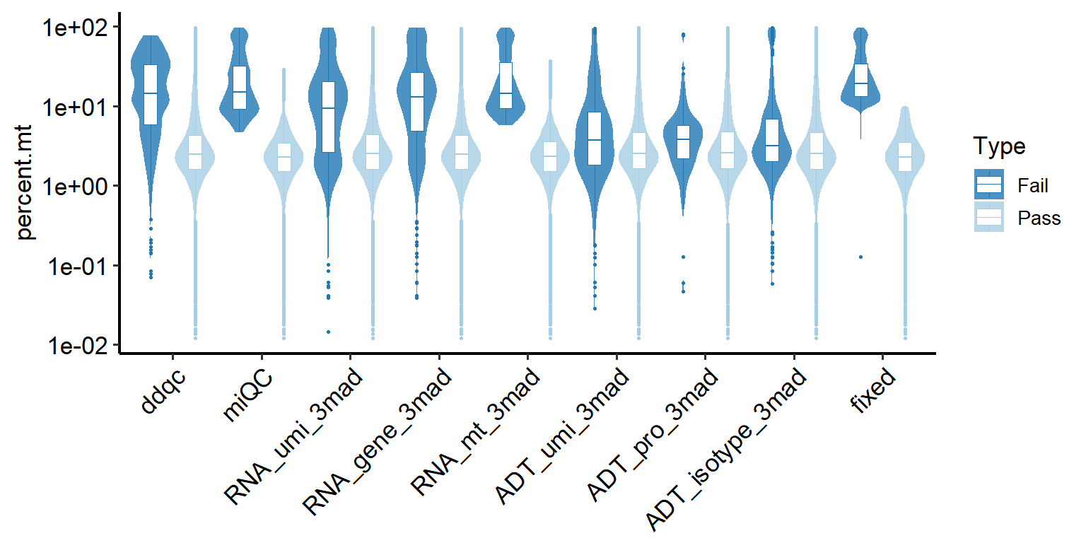
# Plotting comparison of low-quality cell detection methods (each sample).
# Choose the column representing your sample for the `split.by` parameter.
out <- PlotCellMethodVln(pbmc, metrics.by = "percent.mt", type.detection = "lq", split.by = "orig.ident")
names(out)
## [1] "TP1" "TP2" "TP3" "TP3-rep"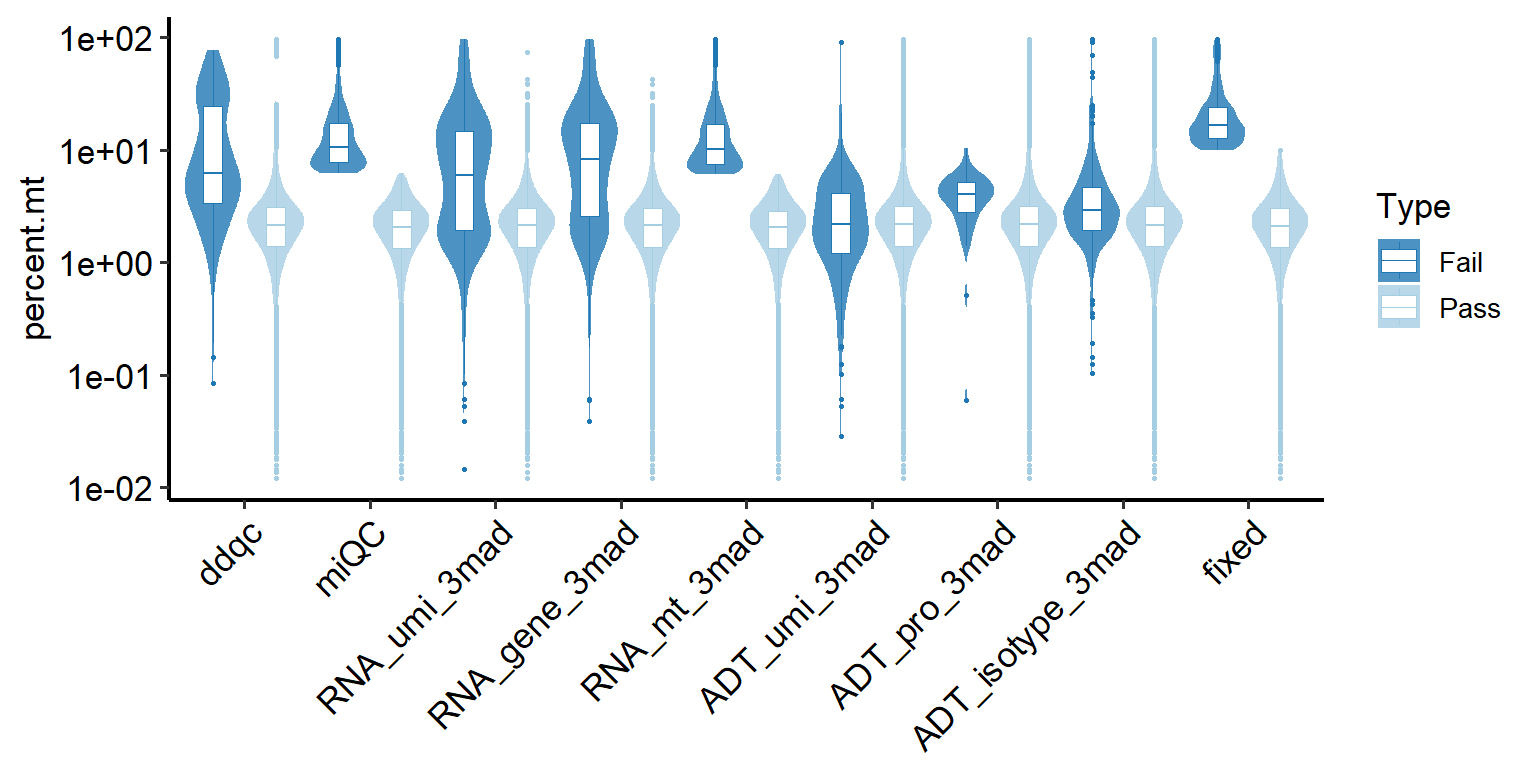
4.5.4 Visualization of scatter plots for cell metrics
You can view two metrics simultaneously in 2D mode.
# Overall visualization of cell metrics
PlotCellMetricsScatter(pbmc, metrics.by = c("percent.mt", "nFeature_RNA") , log.x = T, log.y = T)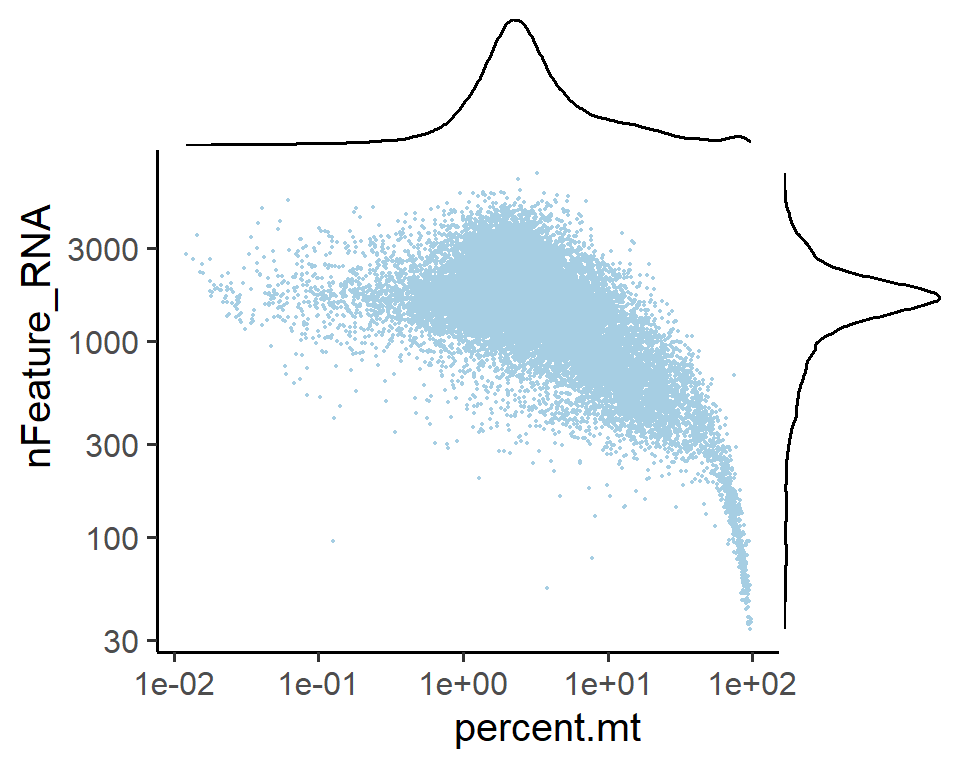
# Visualization of cell metrics for certain detection method, like `lq_fixed`
PlotCellMetricsScatter(pbmc, metrics.by = c("percent.mt", "nFeature_RNA") , log.x = T, log.y = T, group.by = "lq_fixed")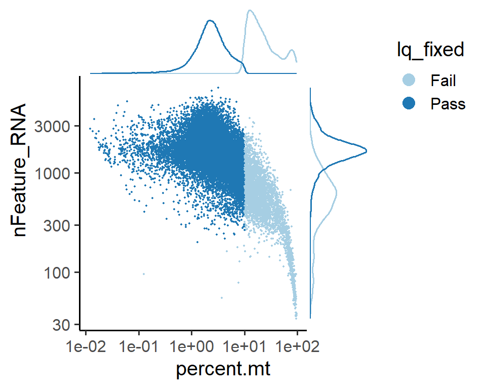
# Visualization of cell metrics for certain detection method in each sample
# PlotCellMetricsScatter(pbmc, metrics.by = c("percent.mt", "nFeature_RNA") , log.x = T, log.y = T, group.by = "lq_fixed", split.by="orig.ident")
You can view three metrics simultaneously in 3D mode.
# Overall visualization of cell metrics
PlotCellMetricsScatter(pbmc, metrics.by = c("percent.mt", "nFeature_RNA","nCount_RNA") , log.x = T, log.y = T)4.6 Filter out problematic droplets or cells
After executing the above steps, you can choose the filtering strategy you need. For example, you can select the results from lq_RNA_mt_3mad and db_scDblFinder to filter out the cells marked as Fail.
pbmc <- FilterCells(pbmc, filter_columns = c("lq_RNA_mt_3mad", "db_scDblFinder"),
                    filter_logic = "or")
If you want to filter out the Fail cells that are in the intersection of multiple methods, such as db_scDblFinder and db_hybrid, you can change the filter_logic to “and”.
If you want to return the specific count values of each sample before and after filtering, take lq_RNA_mt_3mad for example.
out <- FilterCells(pbmc,  filter_columns = c("lq_RNA_mt_3mad", "db_scDblFinder"),
                   filter_logic = "or", return.table = T, split.by = "orig.ident")
## Total cells before filtering: 28498
## Total cells after filtering: 23344
## >>>> Sample: TP1
##   Cells before filtering: 10136
##   Cells after filtering: 8549
## >>>> Sample: TP2
##   Cells before filtering: 9063
##   Cells after filtering: 7220
## >>>> Sample: TP3
##   Cells before filtering: 3697
##   Cells after filtering: 3023
## >>>> Sample: TP3-rep
##   Cells before filtering: 5602
##   Cells after filtering: 4552
out
##    Sample Before_Filtering After_Filtering
## 1   Total            28498           23344
## 2     TP1            10136            8549
## 3     TP2             9063            7220
## 4     TP3             3697            3023
## 5 TP3-rep             5602            4552