5 Feature QC
Compiled: 2025-05-08 Written by Shuting Lu and Daihan Ji
library(SingleCellMQC)
library(BPCells)
#Load a pre-existing Seurat object or process raw data using SingleCellMQC.
pbmc <- readRDS("/data/pbmc.rds")
The main tasks of feature-level QC include:
- Feature quality assessment- Focused on identifying and removing low-expression features with abnormal variability.
- Systematic background noise correction- Aimed at detecting and removing contaminations from ambient RNA and nonspecific antibody binding.
5.1 Feature quality assessment
The feature quality assessment module in SingleCellMQC calculates QC metrics for both RNA and surface protein (ADTs) features.
For RNA, key metrics include average expression level, expression standardized variance, and the detection rate across all cells.
For surface protein features (ADTs), QC metrics include the detection rate of each antibody-derived tag across cells, expression level, expression standardized variance.
5.1.1 Calculating feature metrics
The first step in this module is to calculate the relevant metrics for the feature and adjust the option of adding it to the Seurat object.
If no SeuratObject is added, sample.by is the sample column that can be selected, and the result will return the outcome of the metric calculation for each sample and for all samples. If several samples result in a large amount of data, it is recommended to store them separately to avoid the original Seurat object taking up too much space.
# Without adding the Seurat object
feature_metrics <- CalculateMetricsPerFeature(pbmc, add.Seurat = F, sample.by="orig.ident")
# With the addition of the Seurat object
pbmc<- CalculateMetricsPerFeature(pbmc, add.Seurat = T, sample.by="orig.ident")
Where can you view the results of feature-level QC?
You can explore them in pbmc@misc[["SingleCellMQC"]][["perQCMetrics"]][[perFeature]].
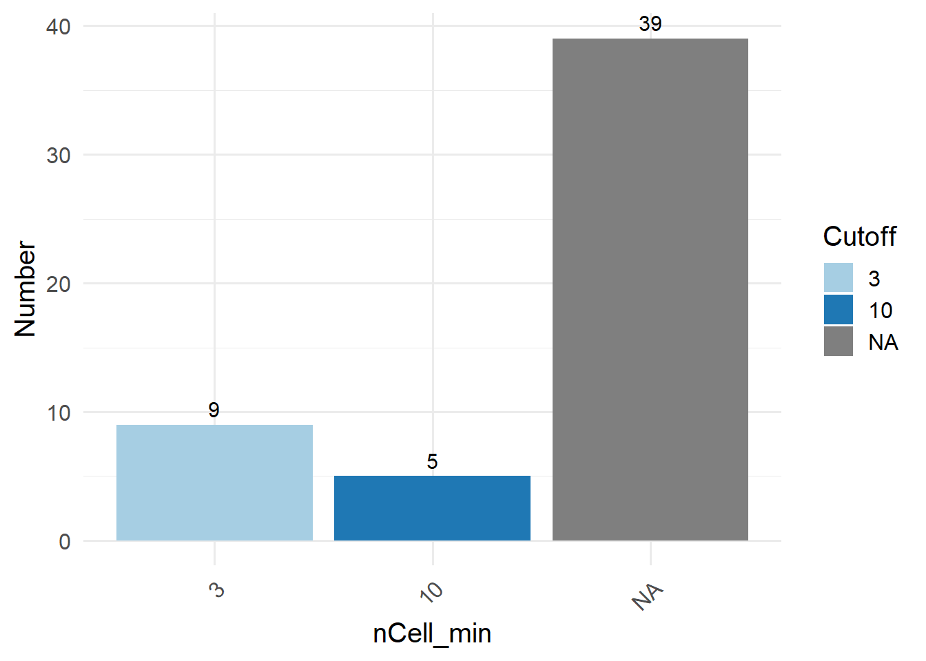
5.1.2 Reference QC thresholds for feature QC
To filter low-quality features, SingleCellMQC offers the values for the minimum number of cells in which a feature is detected (nCell). These thresholds were determined using an integrative analysis of 240 public single-cell studies spanning 11 human tissues to adapt to different tissue types.
5.1.3 Calculating per-feature variance explained by batch factors
In this module, it supports identifying the potential genes/proteins that are most affected by batch factors or individual effects by calculating ANOVA-derived R² values.
# Calculating per-feature variance explained by batch factor (Batch_TotalSeq_C_Antibodies).
Seurat::DefaultAssay(pbmc) <- "ADT"
out <- RunVarExplained(pbmc, assay = "ADT", variables = c("Batch_TotalSeq_C_Antibodies"))
# View of inter-individual top 10 influence level genes
PlotVEPerFeature(out, plot.type="bar")
## $Batch_TotalSeq_C_Antibodies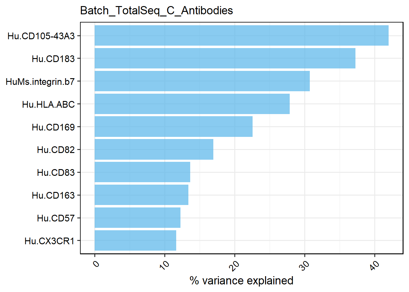
# interactive table
PlotVEPerFeature(out, plot.type="bar", return.type = "interactive_table", ntop = 10)Variance Explained per Feature (top 10)
5.1.4 Base plots of feature metrics
Select the metric category to be displayed, such as type=“pct”, type=“variance.standardized”, etc. Visualisations such as density plots, bar graphs and interactive tables can be selected by specifying the “return.type”.
# Density and bar graphs
PlotFeatureMetrics(feature_metrics, type="variance.standardized", return.type = "plot", sample = "All")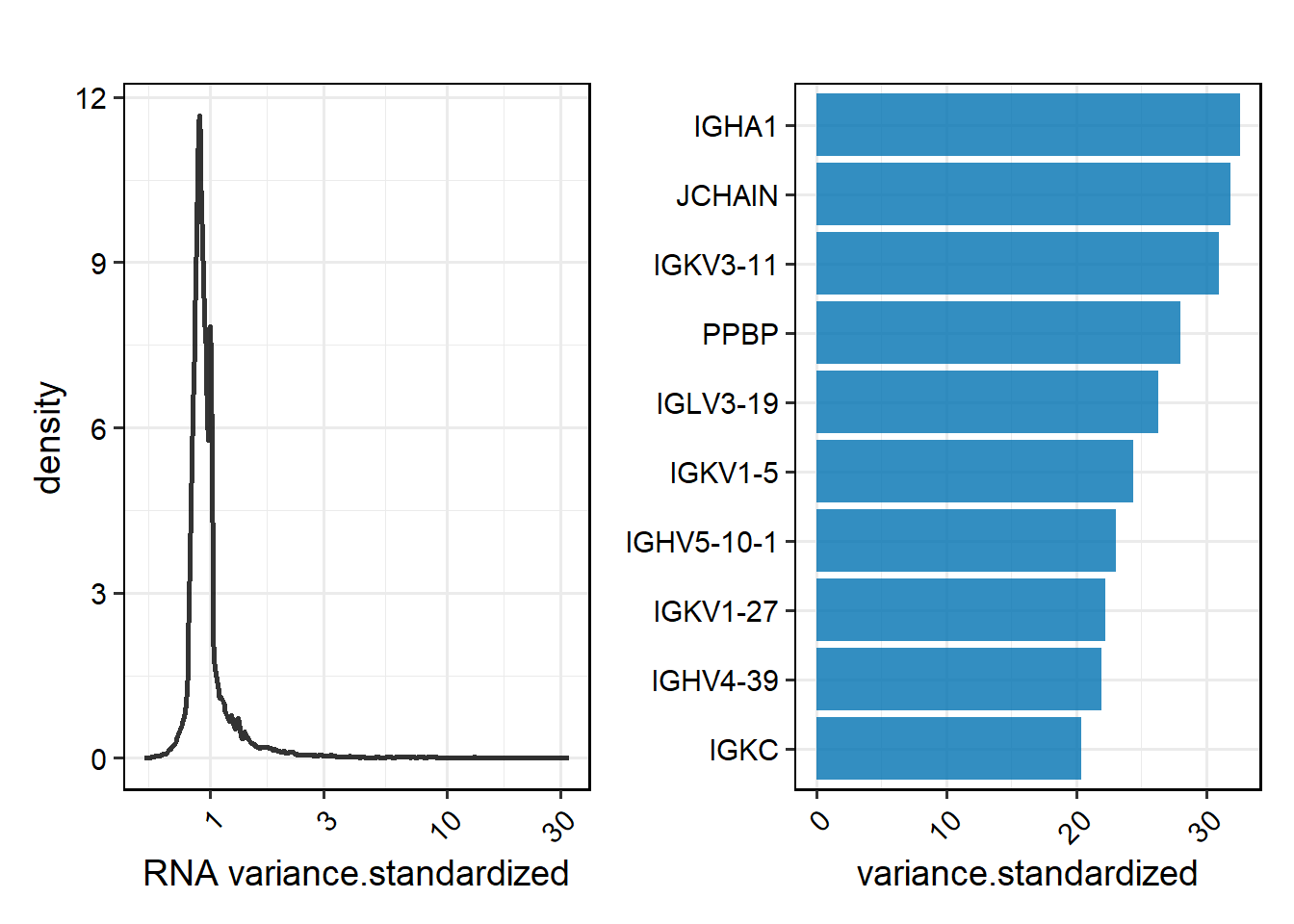
# Metrics visualisation of Feature for specified samples.
PlotFeatureMetrics(feature_metrics, type="pct", return.type = "plot", sample = "TP1")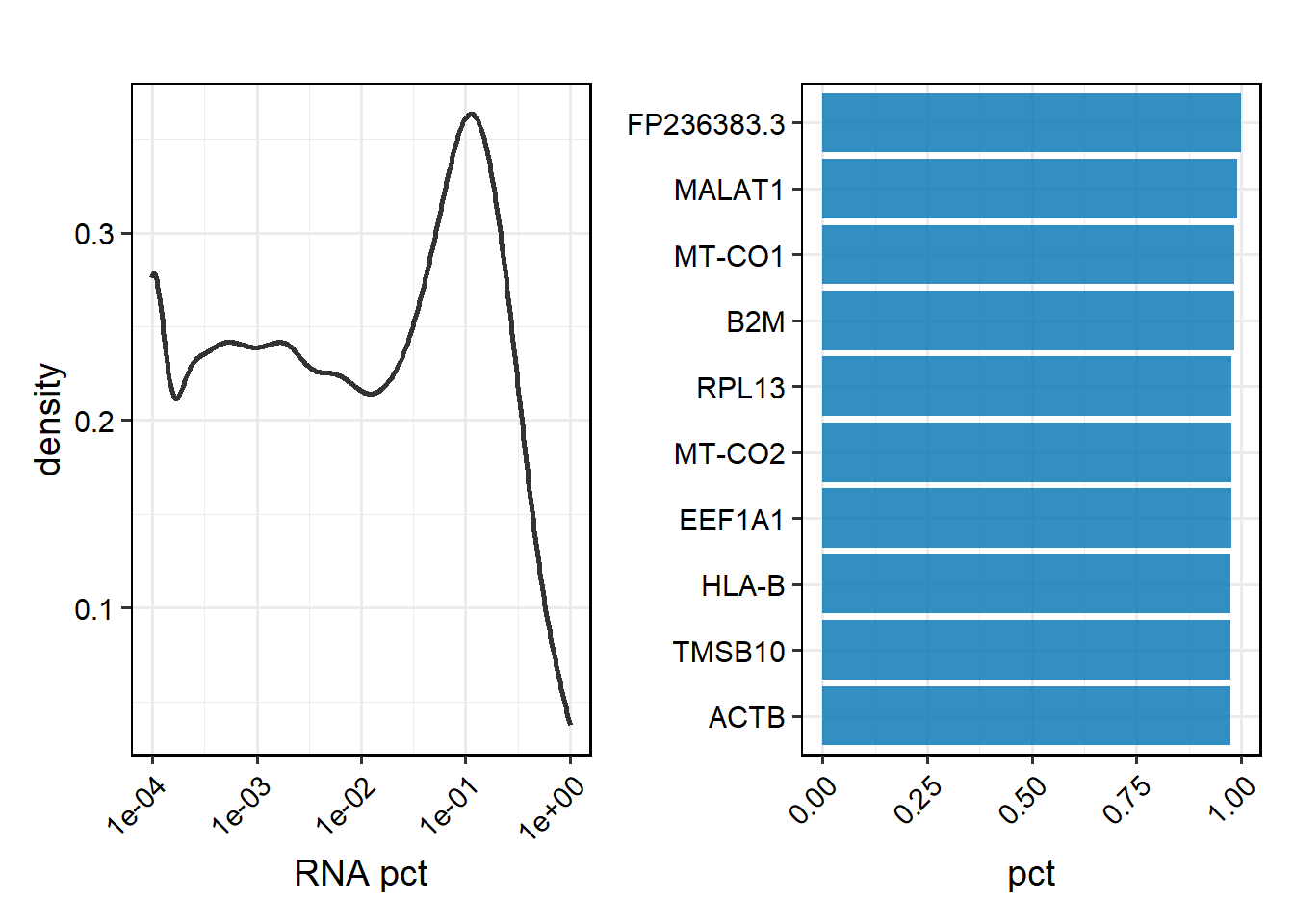
5.1.5 Scatter plot of the feature metrics
Specify the number of metrics to plot and choose between 2D and 3D in the Scatter plot.
- In a 3D scatterplot, the entire graph can be freely rotated. This makes it easier to see the relationships between individual metrics.
# 2D Scatterplot
PlotFeatureMetricsScatter(feature_metrics, metrics.by = c("pct", "mean"), sample = "TP1")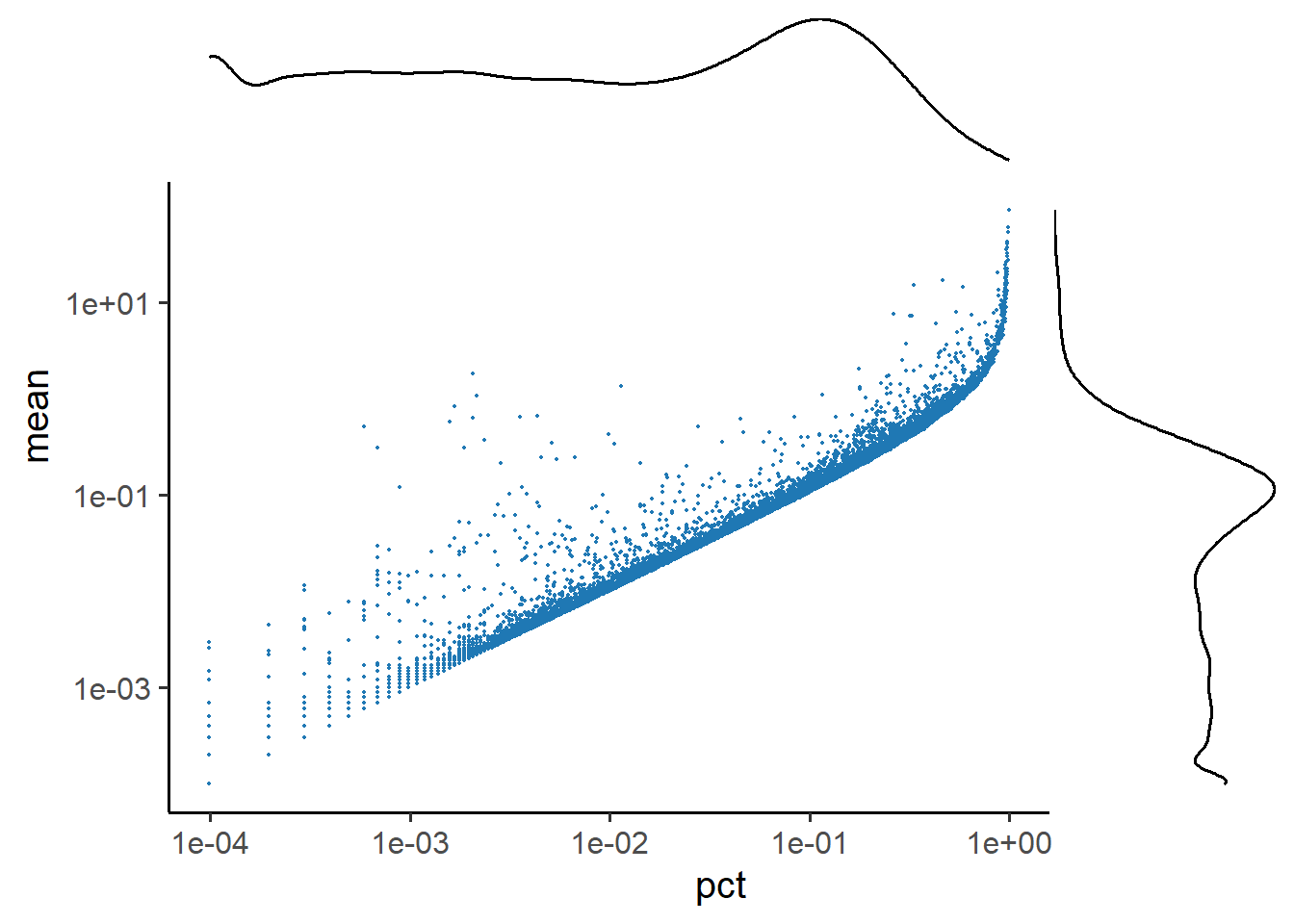
5.2 Systematic background noise correction
To address contamination from sources such as ambient RNA or nonspecific antibody binding, SingleCellMQC employs the ‘RunCorrection’ function for background noise correction using DecontX for RNA and DecontPro for ADT. For more targeted correction, this function also integrates scCDC to identify and remove highly contaminated RNAs or proteins, minimizing the risk of overcorrecting unaffected features.
5.2.1 scCDC
Firstly the included features are detected, where group.by refers to the column name of the clustering, so before executing this function, you should clustering the clusters, for example by running the RunPipelinePerGroup() function.
# If you do not have pre-existing cell clustering information, you can run RunPipeline or RunPipelinePerGroup to obtain cluster labels
# RunPipeline per sample
pbmc_list <- RunPipelinePerGroup(pbmc, preprocess = "rna.umap")

# Contaminated features detection per sample
HCF_out <- FindContaminationFeature(pbmc_list, assay= "RNA", group.by="seurat_clusters", restriction_factor=0.5, split.by = "orig.ident")
Perform background corrections on genes by entering the names of the genes to be corrected as features. These features can be global corrections based on HCF_out or partial corrections based on custom feature names.
# RunCorrection_scCDC per sample based on HCF_out
# Correct <- RunCorrection_scCDC(pbmc_list, assay= "RNA", features=HCF_out, split.by = "orig.ident" )

# RunCorrection_scCDC per sample based on custom features
Correct <- RunCorrection_scCDC(pbmc_list, assay= "RNA", features= c("CD3D", "CD3E", "CD79A"), split.by = "orig.ident" )
Although this method is designed for RNA data correction, it also performs well in the correction of ADT data in our PBMC dataset.